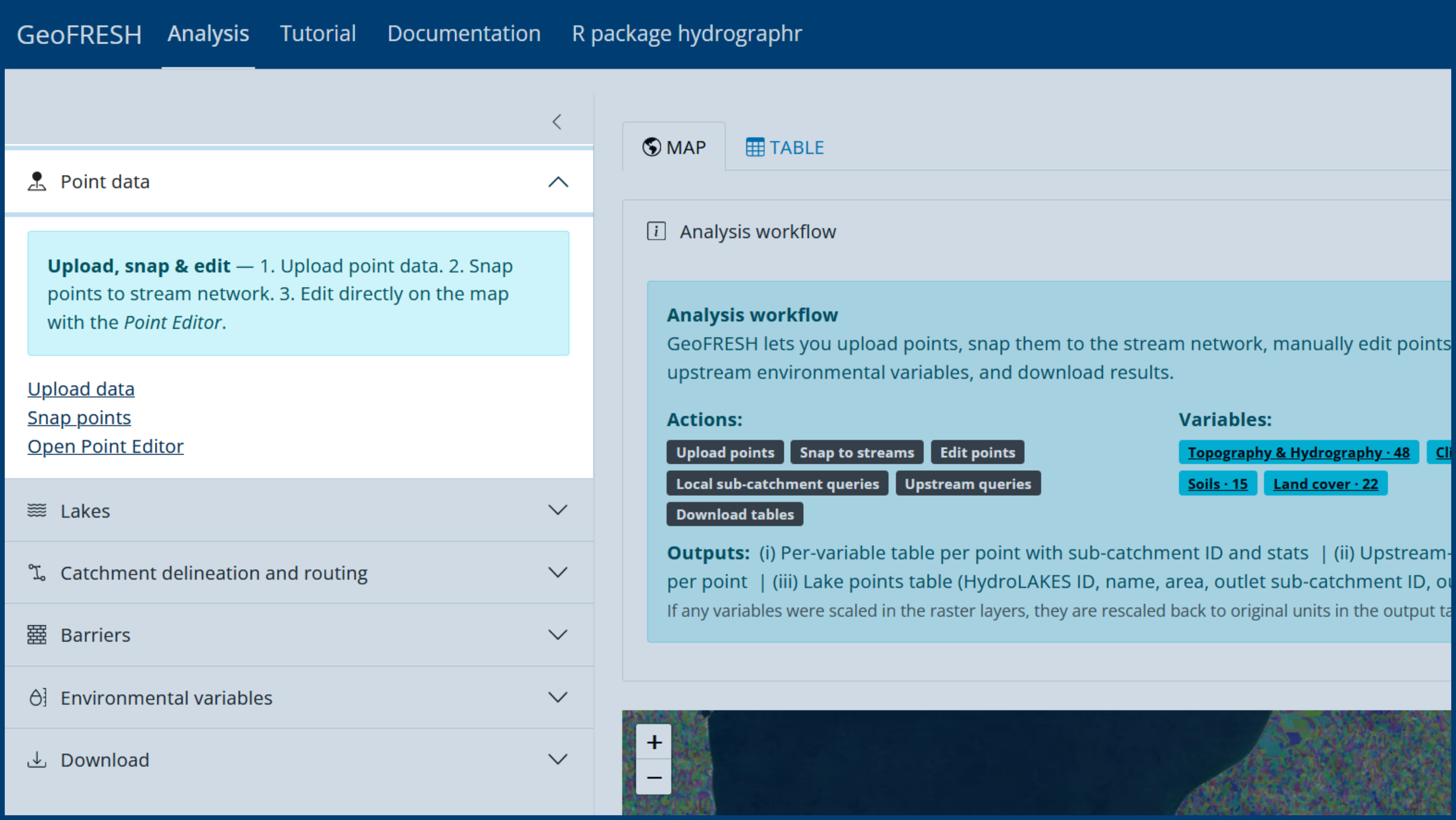
GeoFRESH lets you upload points, snap them to the stream network, manually edit points, query local and upstream environmental variables, and download results.
This tutorial walks though the single steps of GeoFRESH using the test data set (random selection of fish occurrences, drawn from the Harmonised freshwater fish occurrence and abundance data for 12 federal states in Germany, downloaded from GBIF).
GeoFRESH helps you link point locations (e.g., occurrence records or sampling sites) to the Hydrography90m river network and catchments, and then annotate those points with environmental variables at two scales: local sub-catchment and upstream catchment.
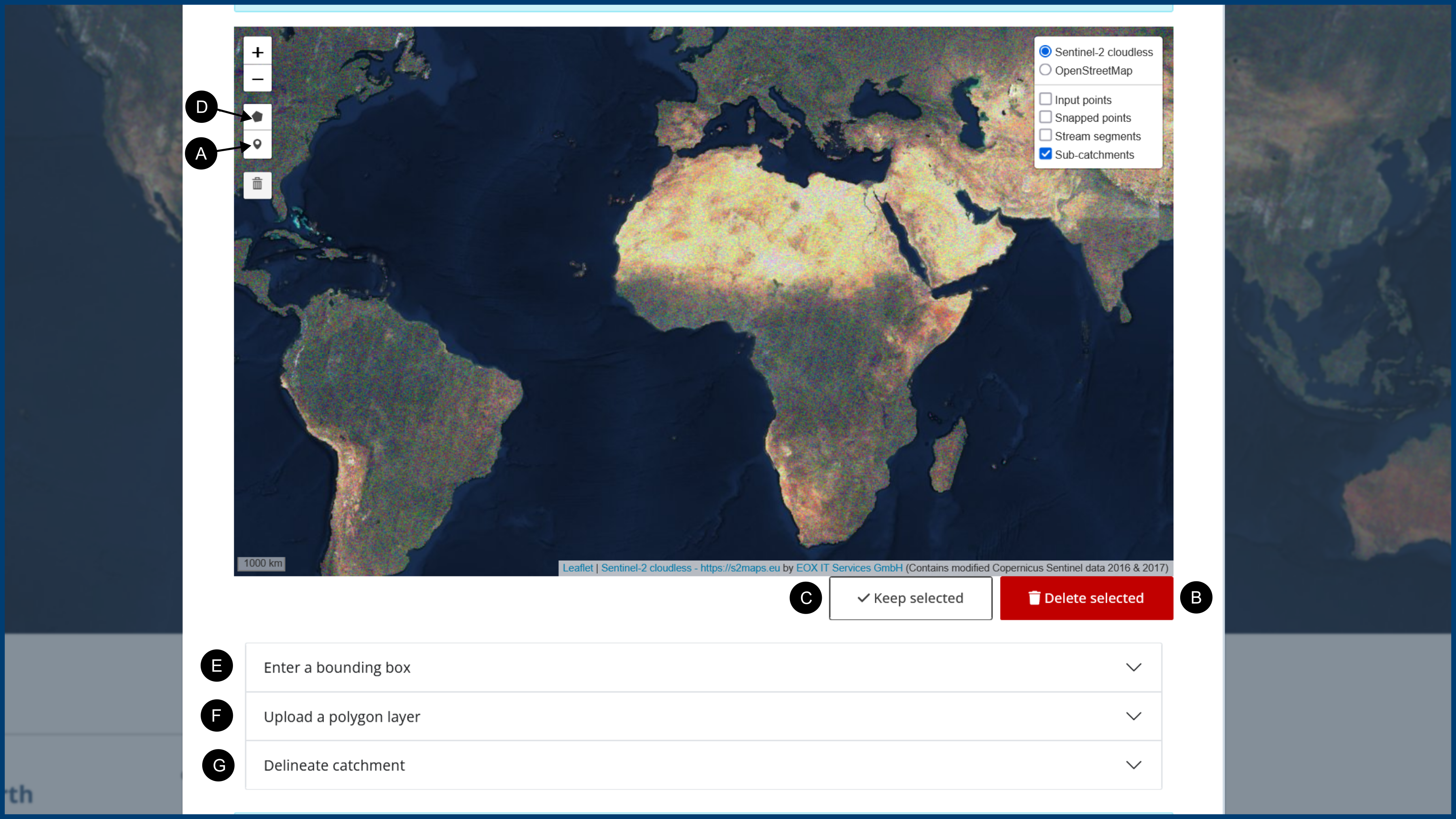
Point data can be created either by uploading a CSV or by creating/editing points in the Point Editor (Figure 1). Depending on your needs, you can follow one of several workflows.
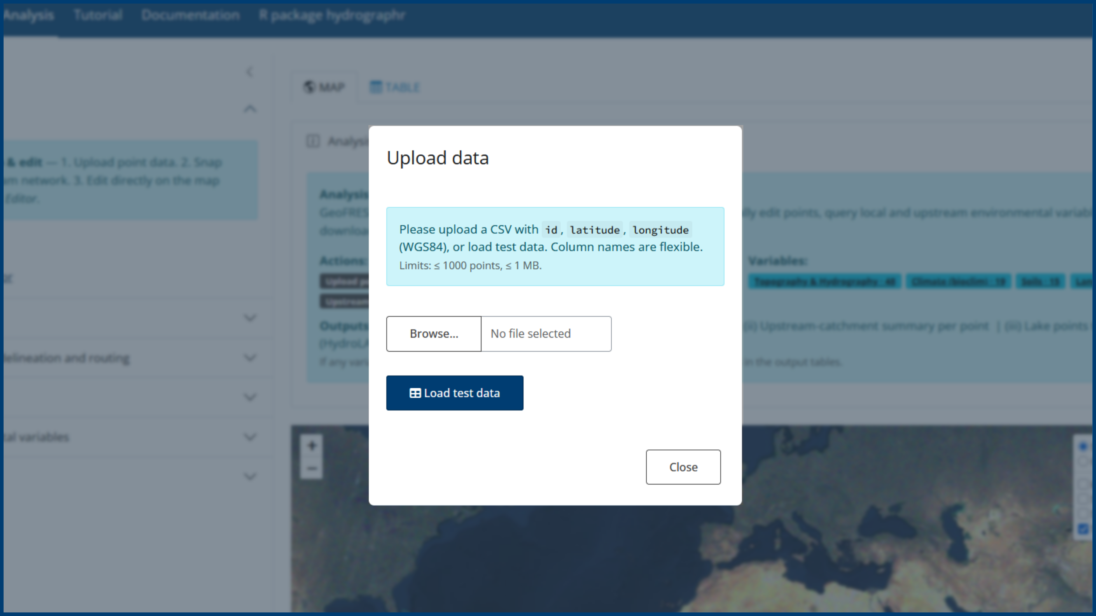
Upload a .csv file containing point coordinates. The file must include:
Column names are flexible, but coordinates must be in WGS84 (EPSG:4326).
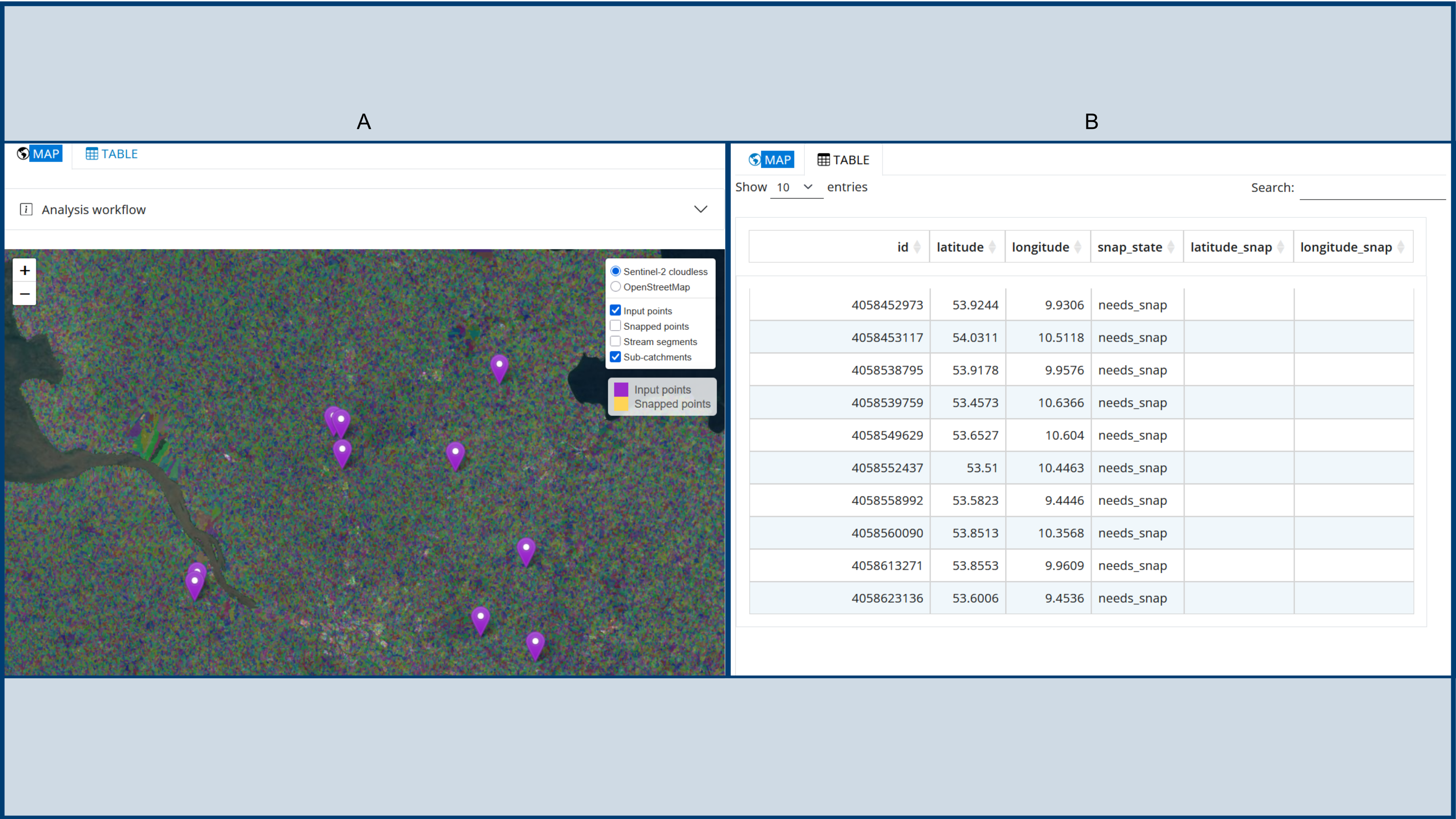
After upload:
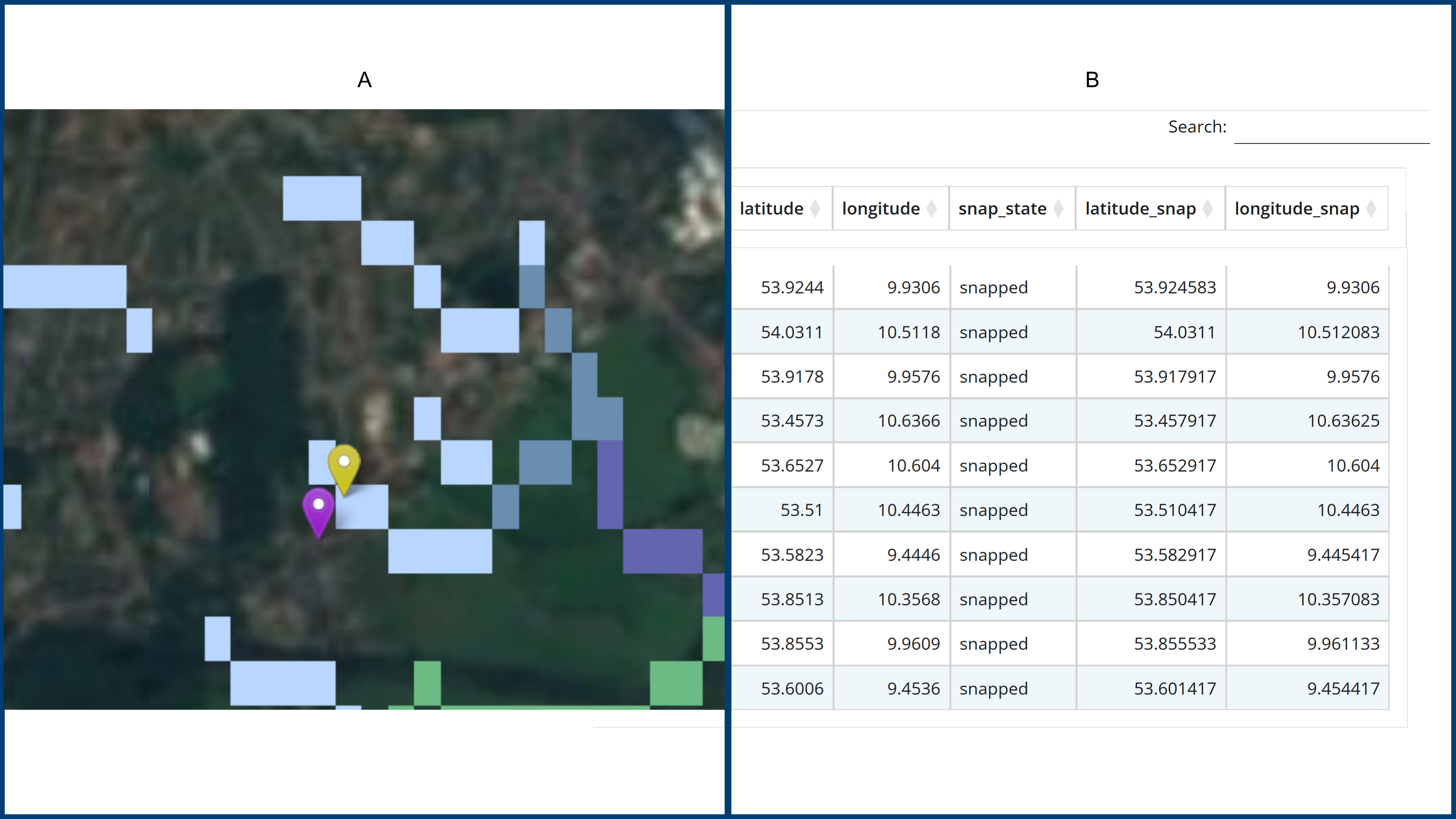
Open the Point Editor (Figure 1) to create or refine points interactively:
This option is useful for digitizing points manually or correcting uploaded coordinates.
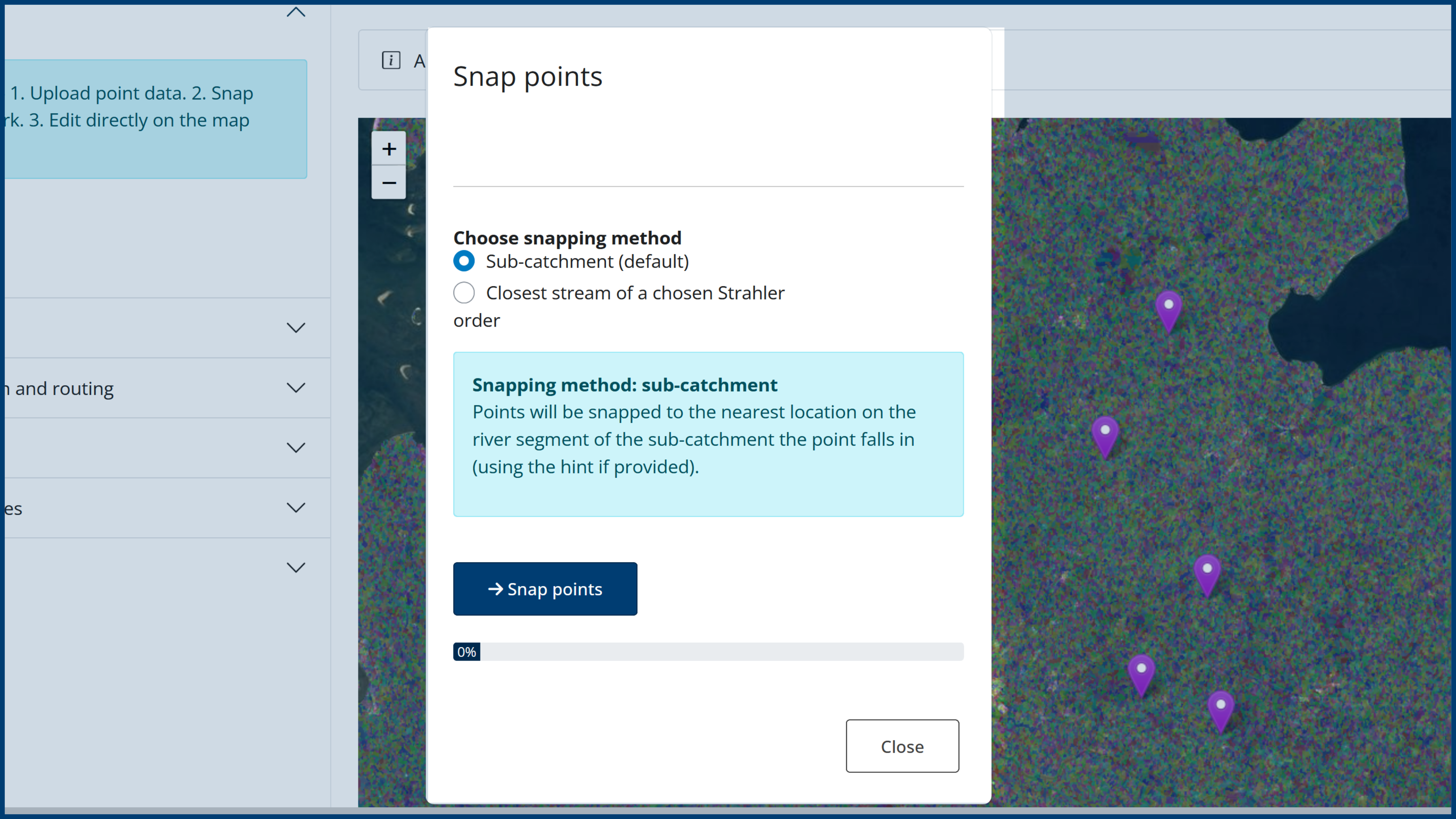
Snapping assigns each point to the Hydrography90m regional unit, sub-catchment, and stream segment, and places the point exactly on the stream line. A progress bar indicates status.
GeoFRESH provides two snapping methods (Figure 5):
Sub-catchment snapping (default)
Points are snapped to the nearest stream segment within the sub-catchment the point falls into.
Closest stream by Strahler order (optional)
Points are snapped to the nearest stream segment with a selected Strahler order, within a maximum search distance. Points farther than the maximum distance remain unsnapped.
After snapping:
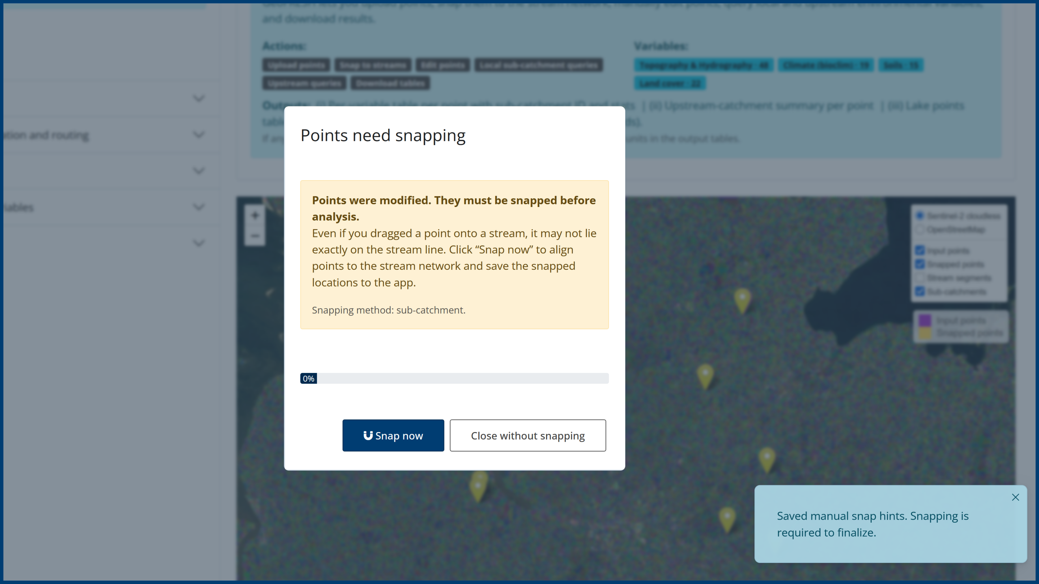
Manual correction concept (important): If the initial snapping result is not what you expect, you can correct it in the Point Editor:
Afterwards, you can annotate the point data with environmental information across the sub-catchment of each point. You can select from a suite of 48 variables related to
topography and hydrography,
19 climate variables (i.e., current bioclimatic variables),
15 soil variables, and
22 land cover variables.
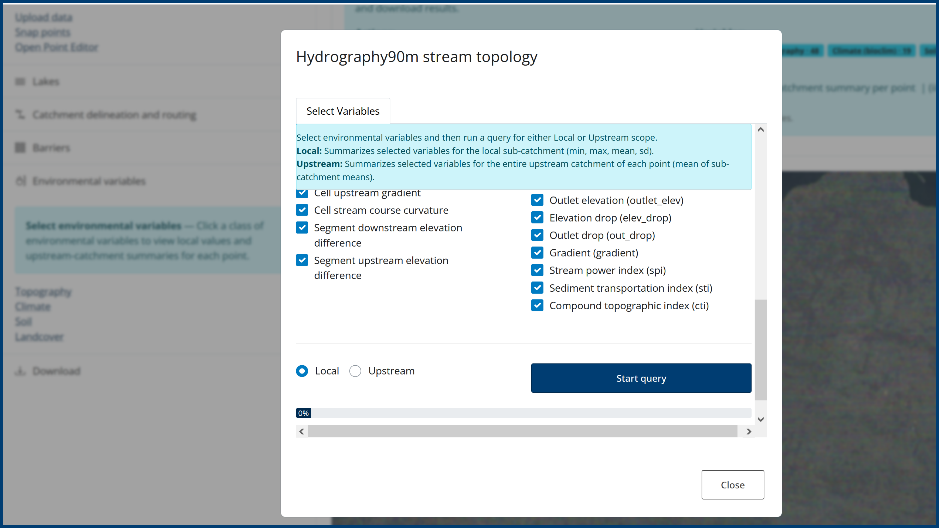
You can compute summaries for:
Click Start query to compute the results (Figure 8).
Each extraction (local or upstream) provides:
Results table (CSV)
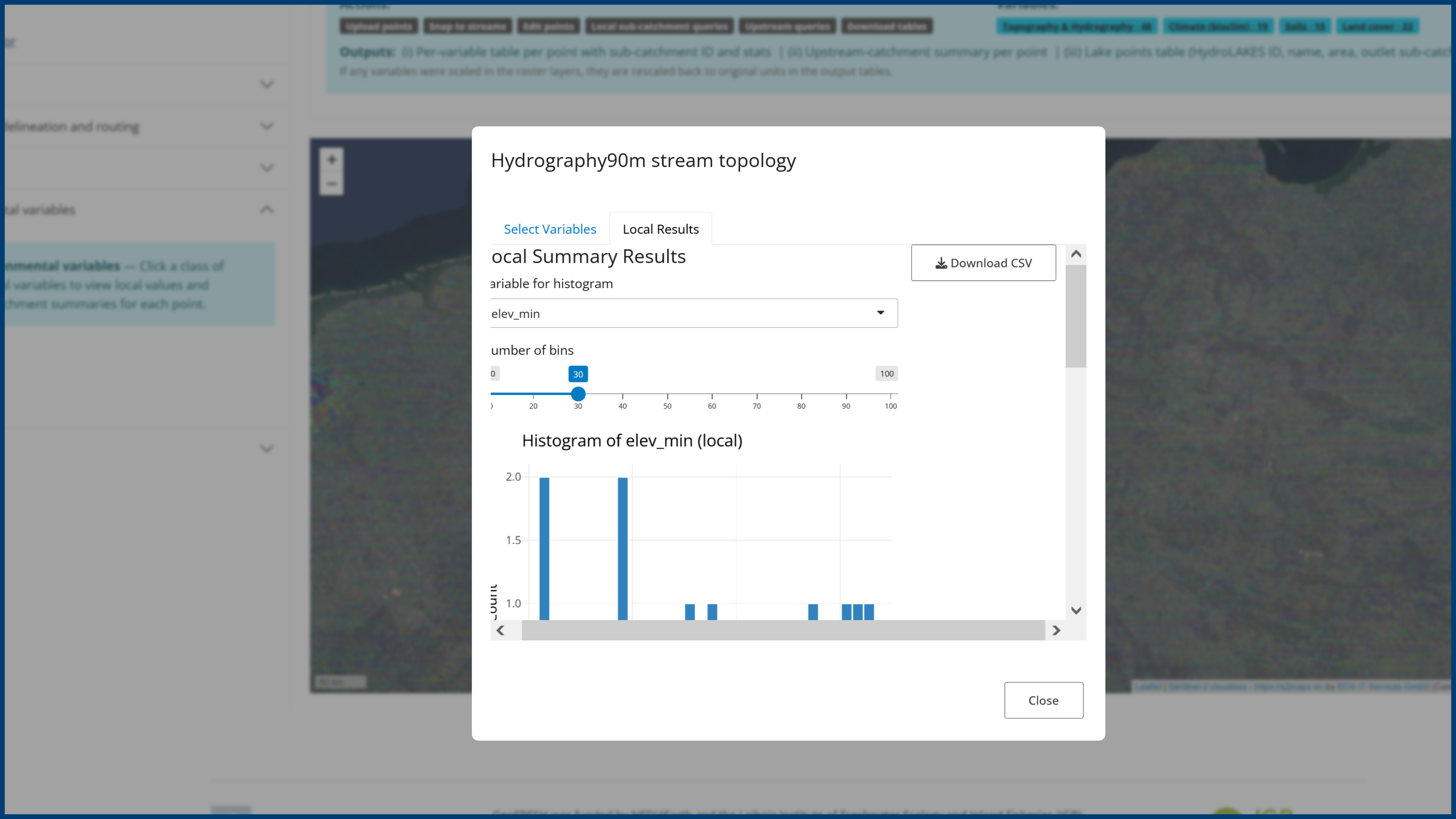
A table is generated and can be downloaded as a CSV file from the same menu where the extraction was run (Figure 9).
Summary plot
A plot (Figure 9) is produced to summarize the selected variables (e.g., distributions for continuous variables and category summaries for categorical land-cover variables). This helps with quick interpretation and quality control before downloading.
GeoFRESH provides multiple download options depending on what you produced in the session.
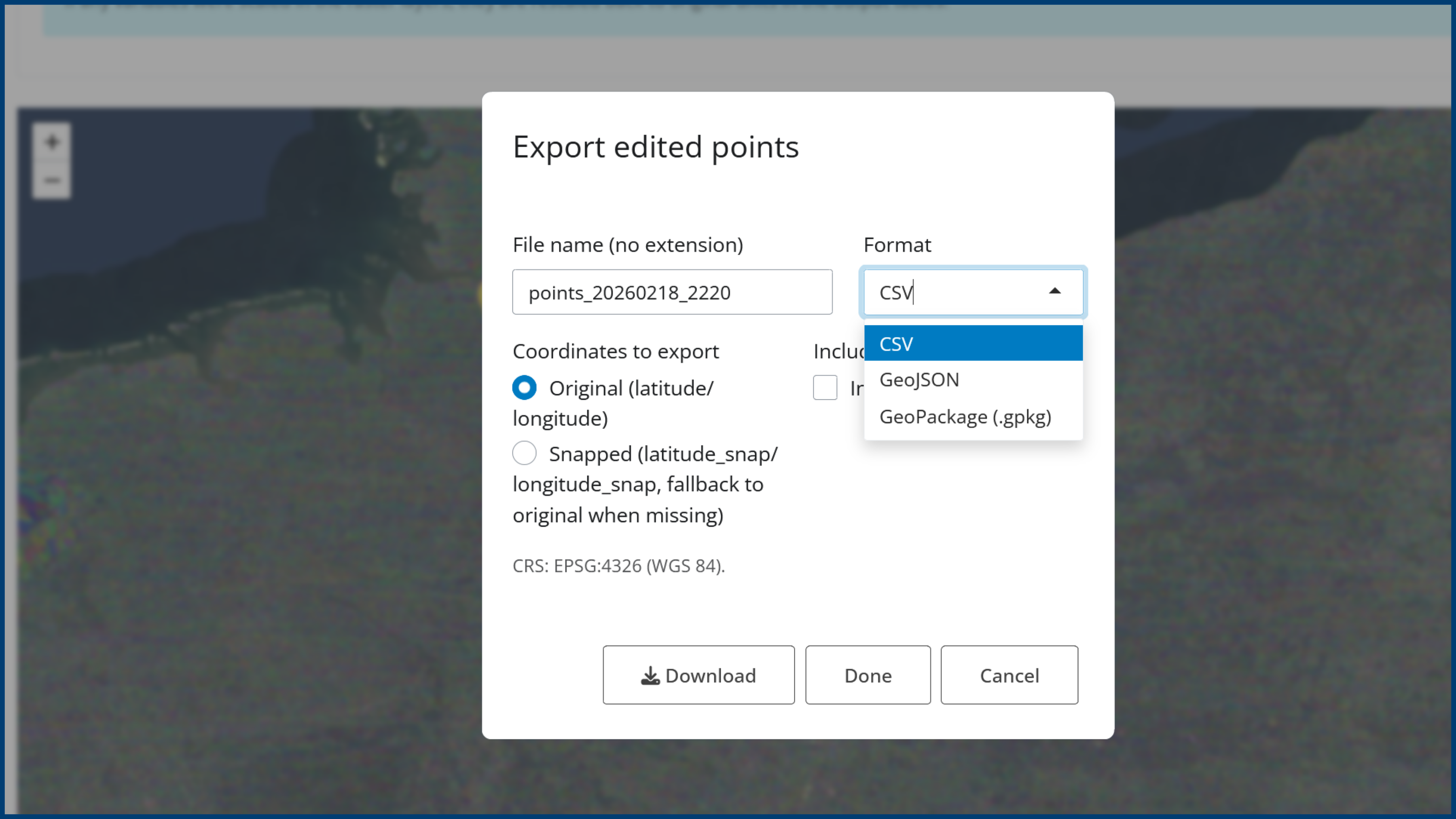
From the Point Editor, use Save as… to export a points file at any time (Figure 10). You can export:
Local and upstream environmental annotation tables can be downloaded as CSV directly from the menu where they were created (Figure 9).
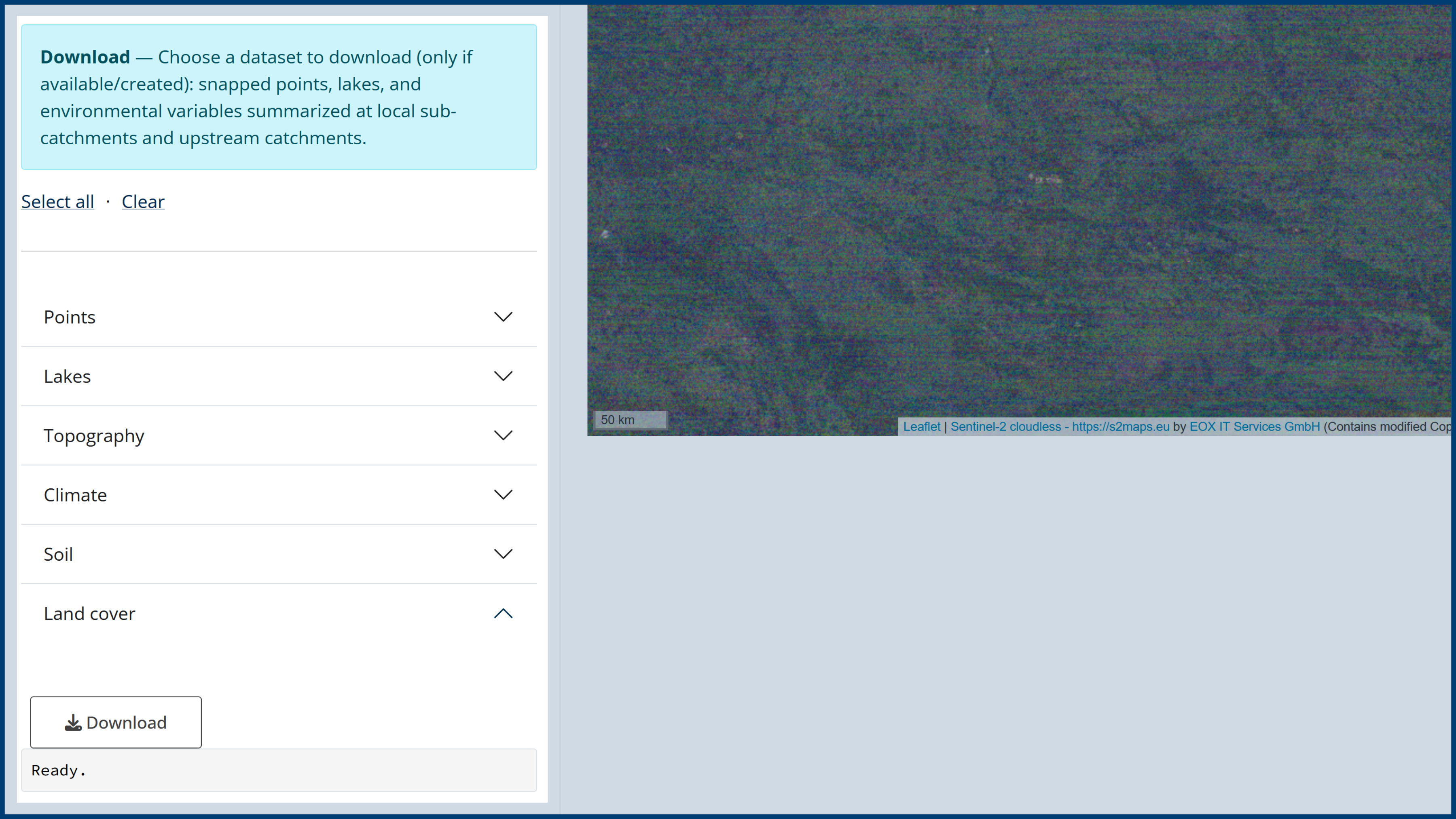
A central Download menu (Figure 11) in the lateral sidebar allows you to download:
This is the easiest way to retrieve all outputs in one place.
Use this workflow when default snapping produces the expected results.
Use this workflow when you need interactive correction to achieve the intended stream placement.
Use this workflow when you want to build a dataset from scratch inside GeoFRESH.
All data are session-based. When you close the browser window, uploaded data and derived results are removed. No data are stored permanently on the platform.
GBIF.org (24 April 2023) GBIF Occurrence Download. doi.org/10.15468/dl.xbuqe5
Freshwater water bodies are highly connected with each other and with their terrestrial catchments. In the light of climate and land use changes as well as feedback mechanisms between earth systems, the integration of earth system data into freshwater research is long-overdue to assess those interdependencies. However, freshwater-specific characteristics like spatial connectivity and fragmentation as well as legacy effects require a specialized workflow. Within the first pilot project “GeoFRESH: Getting freshwater spatio-temporal data on track”, the aim was to built a prototype for a new online platform, called GeoFRESH. The platform provides the integration, processing, management and visualization of various standardized spatiotemporal freshwater-related earth system data. The platform is built around IGB GeoNode using RShiny and includes the newly created Hydrography90m dataset. In the second pilot project “Connecting rivers and lakes FAIRly” we integrated lakes into GeoFRESH, currently based on the Hydrolakes dataset and planned to be replaced by the NASA SWOT data. The aim for the third pilot project “The seamless interoperability of geospatial freshwater tools” is an improved interoperability and user experience of the GeoFRESH platform, including interactive point snapping, an improved visualization, a connection to the hydrographr R-package, and the integration of dams / barriers.
Development team: Vanessa Bremerich, Yusdiel Torres-Cambas, Afroditi Grigoropoulou,
Jaime R. García Márquez, Sami Domisch, Thomas Tomiczek, Merret Buurman
Proposal team: Sami Domisch, Giuseppe Amatulli, Luc De Meester, Hans-Peter Grossart,
Mark Gessner, Thomas Mehner, Vanessa Bremerich, Rita Adrian
Contact information: sami.domisch@igb-berlin.de
Source code:
github.com/glowabio/geofresh
License of the source code:
GPL-3.0 license
Bug reports and feature requests:
github.com/glowabio/geofresh/issues
Project duration:
Pilot 1: 01.04.2022 - 31.03.2023
Pilot 2: 01.10.2023 - 30.09.2024
Pilot 3: 01.03.2025 - 28.02.2026
Project funding:
NFDI4Earth (DFG)
This work has been funded by the German Research Foundation (DFG) through the project NFDI4Earth (TA1 M1.1, DFG project no. 460036893, www.nfdi4earth.de) within the German National Research Data Infrastructure (NFDI, www.nfdi.de).
Please cite the GeoFRESH platform as follows:
Domisch, S., Bremerich, V., Buurman, M., Kaminke, B., Tomiczek, T., Torres-Cambas, Y., Grigoropoulou, A., Garcia Marquez, J. R., Amatulli, G., Grossart, H. P., Gessner, M. O., Mehner, T., Adrian, R. & De Meester, L. (2024). GeoFRESH – an online platform for freshwater geospatial data processing. International Journal of Digital Earth, 17(1). doi.org/10.1080/17538947.2024.2391033
In addition, GeoFRESH relies on a number of external data sources regarding the environmental data and we ask you to please use the following citations depending on your analysis:
Topography (Hydrography90m)
Amatulli, G., Marquez, J.G., Sethi, T., Kiesel, J., Grigoropoulou, A., Ublacker,
M. M., Shen, L. Q., & Domisch, S. (2022). Hydrography90m: a new high-resolution
global hydrographic dataset. Earth System Science Data, 14(10), 4525-4550.
doi.org/10.5194/essd-14-4525-2022
Climate (CHELSA v2.1)
Karger, D.N., Conrad, O., Böhner, J., Kawohl, T., Kreft, H., Soria-Auza, R.W.,
Zimmermann, N.E., Linder, P., Kessler, M. (2017): Climatologies at high resolution
for the Earth land surface areas. Scientific Data, 4 170122.
doi.org/10.1038/sdata.2017.122
Karger, D.N., Conrad, O., Böhner, J., Kawohl, T., Kreft, H., Soria-Auza, R.W.,
Zimmermann, N.E., Linder, H.P. & Kessler, M. (2021) Climatologies at high resolution
for the earth’s land surface areas. EnviDat.
doi.org/10.16904/envidat.228.v2.1
Soil (SoilGrids250m)
Hengl, T., Mendes de Jesus, J., Heuvelink, G.B.M., Ruiperez Gonzalez, M.,
Kilibarda, M., Blagotić, A., Shangguan, W., Wright, M.N., Geng, X.,
Bauer-Marschallinger, B., Guevara, M.A., Vargas, R., MacMillan, R.A., Batjes,
N.H., Leenaars, J.G.B., Ribeiro, E., Wheeler, I., Mantel, S., & Kempen, B. (2017).
SoilGrids250m: Global gridded soil information based on machine learning.
PLOS ONE, 12(2), e0169748.
doi.org/10.1371/journal.pone.0169748
Landcover (ESA CCI LC)
ESA. Land Cover CCI Product User Guide Version 2. Tech. Rep. (2017). Available
at:
maps.elie.ucl.ac.be/CCI/viewer/download/ESACCI-LC-Ph2-PUGv2_2.0.pdf
Lakes (HydroLAKES v1.0)
Messager, M.L., Lehner, B., Grill, G., Nedeva, I., Schmitt, O. (2016).
Estimating the volume and age of water stored in global lakes using a
geo-statistical approach. Nature Communications, 7: 13603.
doi.org/10.1038/ncomms13603
de la Cruz‐Castillejo, L., Cassidy, R., Mitsi, K., Galià‐Camps, C., Benítez‐López, A., Gracia‐Sancha, C., Lorente‐Sorolla, J., Álvarez‐Fernández, A., Mozo, R., Kolomyjec, S., Nichols, S., Manconi, R., Pereira, R., Evans, K., Itskovich, V., Horton, A. L., Leys, S. P., Taboada, S. & Riesgo, A. (2026). Genomic Connectivity and Adaptation Signals of the Freshwater Sponge Ephydatia muelleri Across Its Distribution. Journal of Biogeography 53(1).
doi.org/10.1111/jbi.70142
Mehner, T., Argillier, C., Ferreira, T., Holmgren, K., Jeppesen, E., Kelly, F., Krause, T., Olin, M., Volta, P., Winfield, I. J. & Brucet, S. (2025). Rare fish species in European lakes – patterns and processes. Biodiversity and Conservation 34(5), 1833–1855.
doi.org/10.1007/s10531-025-03046-5
Zare Shahraki, M., Fathi, P., Domisch, S., Bruder, A., Ebrahimi Dorcheh, E., Esmaeili Ofogh, A. & Mehner, T. (2025). Evaluating Environmental Predictors of Fish Community Composition in a Semi‐Arid River System Using a Model‐Based Approach. Ecology of Freshwater Fish 34(3).
doi.org/10.1111/eff.70013
15.11.2024: Changed the unit of the climate CHELSA v2.1 variable “bio4” from
°C to °C/100 (following the CHELSA documentation)
19.08.2024: Publication online available at
doi.org/10.1080/17538947.2024.2391033
Updated tutorial
Minor user interface improvements
NFDI4Earth addresses digital needs of Earth System Sciences. Earth System scientists cooperate in international and interdisciplinary networks with the overarching aim to understand the functioning and interactions within the Earth system and address the multiple challenges of global change. NFDI4Earth is a community-driven process providing researchers with FAIR, coherent, and open access to all relevant Earth System data, to innovative research data management and data science methods.
GeoFRESH was initiated as part of the first cohort of 1-year pilot projects: in a first round in 2020, 14 pilots out of 38 were selected and started in April 2022. In the second round, seven (out of 27) pilots were funded and started in 2023. In the third round, another five pilots were funded, starting in 2025.
For further analyses of your freshwater data, you can use the hydrographr R package that facilitates the download and data processing of the Hydrography90m data (publication in Methods in Ecology and Evolution, website with details and examples, source code on GitHub).
For more details and an overview of the functions, please check the hydrographr panel.
The R package hydrographr provides a collection of R function wrappers for GDAL and GRASS-GIS functions to efficiently work with the newly created Hydrography90m dataset and spatial biodiversity data. The easy-to-use functions process large raster and vector data directly on disk in parallel, such that the memory of R does not get overloaded. This allows creating scalable data processing and analysis workflows in R, even though the data is not processed directly in R. Below is a list of the functions that are implemented in hydrographr while additional functions are currently being developed.
The package was described in a publication in Methods in Ecology and Evolution (doi.org/10.1111/2041-210X.14226). A detailed explanation and examples can be found on its website, and its source code is openly available on GitHub.
Development team: Afroditi Grigoropoulou, Marlene Schürz, Sami Domisch,
Jaime García Márquez, Yusdiel Torres-Cambas, Thomas Tomiczek, Merret Buurman,
Christoph Schürz, Vanessa Bremerich
Contact information: sami.domisch@igb-berlin.de
Bug reports and feature requests:
github.com/glowabio/hydrographr/issues
Project funding:
NFDI4Biodiversity (DFG),
NFDI4Earth (DFG)
This work has been funded as a Use Case of NFDI4Biodiversity (DFG project number 442032008, nfdi4biodiversity.org) within the German National Research Data Infrastructure (NFDI, www.nfdi.de). In addition, this work has been funded by NFDI4Earth (DFG project no. 460036893, www.nfdi4earth.de).
Please cite the hydrographr package as follows:
Schürz, M., Grigoropoulou, A., Garcia Marquez, J.R., Torres-Cambas, Y., Tomiczek, T., Floury, M., Bremerich, V., Schürz, C., Amatulli, G., Grossart, H.-P., Domisch, S. (2023). hydrographr: an R package for scalable hydrographic data processing. Methods in Ecology and Evolution, 14, 2953–2963. doi.org/10.1111/2041-210X.14226
Please also cite the Hydrography90m dataset as follows:
Amatulli, G., Garcia Marquez, J.R., Sethi, T., Kiesel, J., Grigoropoulou, A., Üblacker, M., Shen, L., Domisch, S. (2022). Hydrography90m: A new high-resolution global hydrographic dataset. Earth System Science Data, 14(10), 4525–4550. doi.org/10.5194/essd-14-4525-2022
![]() |
get_tile_id() |
Identifies the ID of the regular tile(s) of the Hydrography90m, where the input points are located. The output IDs are required to download the data using the function download_tiles. |
![]() |
get_regional_unit_id() |
Identifies the ID of the regional unit(s) of the Hydrography90m, where the input points are located. The output IDs are required to download the data using the function download_tiles. |
![]() |
download_tiles() |
Downloads data of the Hydrography90m dataset. |
![]() |
download_test_data() |
Downloads the test data of the Hydrography90m dataset, required to run the examples of the manual. |
![]() |
merge_tiles() |
Merges raster (.tif) or vector (.gpkg) files using the GDAL functions gdalbuilvrt and gdal_translate for raster files and ogrmerge.py and ogr2ogr for vector files. |
![]() |
crop_to_extent() |
Crops a raster (.tif) file to a polygon border line or to the extent of a bounding box using the GDAL function gdalwarp. |
![]() |
snap_to_network() |
Snaps point to the next stream segment within a defined radius or a defined radius and a minimum flow accumulation using the GRASS GIS function r.stream.snap. |
![]() |
snap_to_subc_segment() |
Snaps points to the stream segment of the sub-catchment where the points are located in using the GRASS GIS functions v.net and v.distance. |
![]() |
set_no_data() |
Sets a NoData value to input files using the GDAL function gdal_edit.py. |
![]() |
reclass_raster() |
Reclassifies an integer raster (.tif) layer using the GRASS GIS function r.reclass. |
![]() |
extract_ids() |
Extracts the ID value of the drainiage basin and/or sub-catchment raster layer at given point locations using the GDAL function gdallocationinfo. |
![]() |
report_no_data() |
Reports the NoData value of input files using the GDAL function gdalinfo. |
![]() |
extract_zonal_stat() |
Calculates zonal statistics based on one or more environmental variable raster .tif layers across a set (or all) or sub-catchments in a spatial extent using the GRASS GIS function r.univar. |
![]() |
read_geopackage() |
Loads a .gpkg file, or only part of it, as a data.table, graph, sf, or spatVector object. |
![]() |
get_upstream_catchment() |
Calculates the upstream basin taking each point as the outlet using the GRASS GIS function g.region. |
![]() |
get_distance() |
Calculates the euclidean or within-network distance between points using the GRASS GIS function v.distance or v.net.allpairs. |
![]() |
get_segment_neighbours() |
Reports the up- and/or downstream stream segments that are connected to the input segments within a neighbour order. Provides the option to summarise attributes across these segments. |
![]() |
get_catchment_graph() |
Extracts the upstream, downstrea or entire catchment of the input stream segments from a network graph. |
![]() |
get_distance_graph() |
Calculates the network distance between all input sub-catchment IDs from node to node (outlet of the stream segment). |
![]() |
get_pfafstetter_basins() |
Delineates Pfafstetter sub-basins for the input stream network. |